Massively Distributed Parallel EAs

Initially cEAs were designed to run in massively parallel computers. Nowadays this kind of EAs is still studied in the literature due to theirs special characteristics. As the massively parallel computers are disappearing at present, the majority of the research in these algorithms is focused on the sequential case, because when we try to make parallel implementations of cEAs we find two important difficulties, which are characteristics of cEAs:

• In cEAs there are a large number of sub-algorithms because they have typically one single string in every sub-algorithm.
• These sub-algorithms are tightly connected.

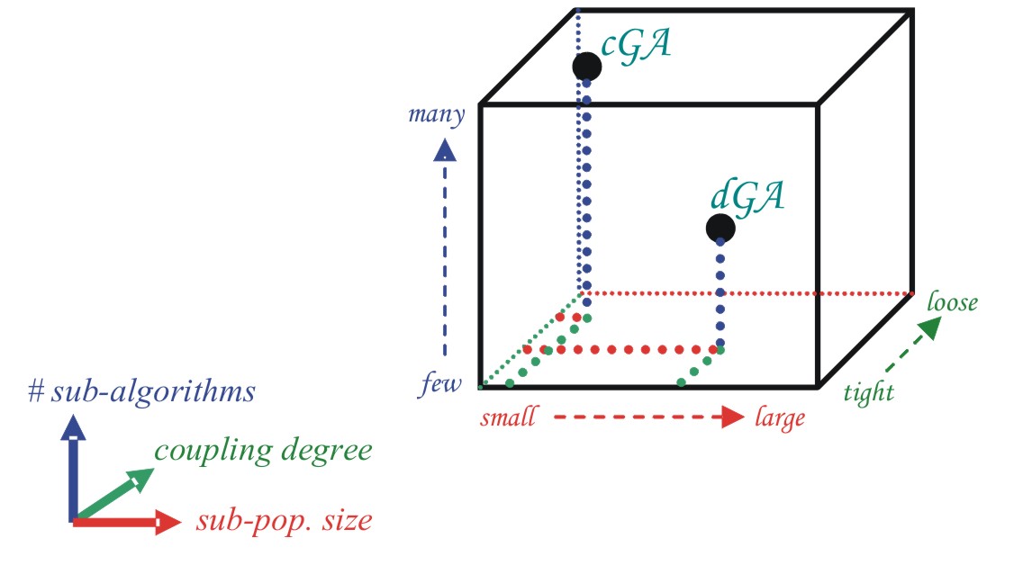
We can see in Figure 1 how cEAs have a very large number of sub-algorithms, with small pop size each and a high coupling degree. In contrast, we can see an easily parallelizable EA -dEA- with smaller number of sub-algorithms running on bigger populations and with medium coupling degree.

Figure 1. The structured-population genetic algorithm cube

However we can find in the literature many studies trying to parallelize cEAs. The motivation for these works are the possibility of facing problems which are limited in CPU, getting better solutions in less time, making profitable the available hardware resources, etc. On the other hand, parallelizing cEAs may be complex because they have a very high connectivity among individuals.

Following we will expose six different strategies for parallelizing fine-grained EAs. The first two approximations are parallel fine-grained panmistic EAs (not decentralized), while the four later correspond to parallel cEAs:

• This first algorithm was proposed by Maruyama, Hirose, and Konagaya in [MHK93]. In this fine-grained algorithm each processor has only one active individual and a buffer to store K suspended individuals. Search in this algorithm progresses by repeating the cycle below (there are no synchronization).
  
  1. Each processor sends out a copy of its active individual to another processor which is selected at random.
  2. For each of the individuals that have arrived from other processors.
     1. One of the suspended individuals in the buffer is deleted according to their relative fitness if the number of the suspended individuals is equal to K.
     2. The newly arrived individual is stored in the buffer.
  3. The recombination operator is applied to the active individual. A part of the active individual is replaced by a part of one of the suspended individuals which have not been used for the recombination yet.
  4. The mutation operator is applied to the active individual.
  5. The active individual is evaluated and compared with the suspended individuals in the buffer.
  6. If the active individual can not survive the selection, one of the suspended individuals is selected according to their relative fitness and exchanged with the active individual.

• This micro grained model is the master and slave model [HMT00]. In this model, simple GA except the evaluation operation is performed in the master processor and transfers the data to the slave processors. The master transfers the data of one gene to one processor and the slave evaluate the fitness of the gene and return the data to the master. Just after the master receive the data from the slave, the master send the data of new gene. This algorithm is summarized in Figure 2.
  

  Forgaty et al.[FH91] reported that this model is very effective when the number of population size is huge. Maruyama et al. [MHK93] developed the efficient program of this model. The advantage of this model is that the program coding is very simple. Even when there are huge number of genes, users need not to change the programs. The other advantage is that it can be easy to keep the load balance. On the other hand, the parallel efficiency does not become 100 %because of the existence of the master CPU. Therefore, when there are not so many processors, it is a very big disadvantage. PGA pack is a free software of this model.

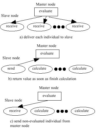  Figure 2. The flow of fine grained model

• This third implementation uses a circularly linked linear ordering of subpopulations [Balu93]. Each subpopulation evolvse only 2 chromosomes per generation. These 2 chromosomes are chosen from a group of 10 chromosomes. The group is comprised of 1 chromosome from each of the four immediate left and 1 chromosome from each of the four immediate right subpopulations, and the 2 chromosomes which were evolved in the subpopulation during the previous generation.

  Each chromosome selected from the neighbors is chosen randomly from the two evolved at each neighbor. The fitness of every chromosome is calculated relative to the other chromosomes in the group of 10. Two chromosomes from the set of 10 are probabilistically chosen for recombination, based upon their relative fitness. The other 8 chromosomes are discarded.

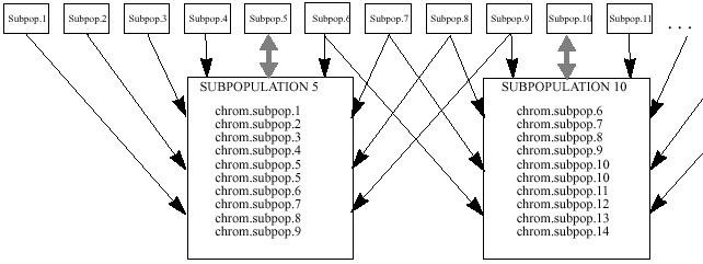Figure 3. Baluja's architecture of subpopulations, arrangement #1. Subpopulation 5 and 10 are shown enlarged. They randomly select 1 chromosome from the 2 chromosomes in each of their 8 closest neighbors, 4 from the left neighbors 4 neighbors, 4 from the right. They also incorporate their own two chromosomes into the population. From this population two chromosomes are probabilistically chosen for breeding. The 8 chromosomes not selected are discarded.

• The fourth implementation uses a two dimensional toroidal array of subpopulations [Balu93]. Each of the subpopulations evolves 2 chromosomes which are chosen from a group of 10. The 8 immediate neighboring subpopulations donate to the group of 10. The remainder of the procedure is completed in the same manner as described above.

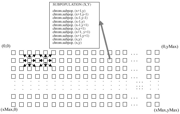Figure 4. Baluja's architecture of subpopulations, arrangement #2. A two dimensional array of processors is assumed. Each processor contributes one of its two chromosomes to each of its 8 nearest neighbors. A sample population for processor (x,y) is shown. The processors are connected in a toroid.

• In the fifth implementation [Balu93], a linear ordering of subpopulations is used once again. One chromosome from each of the 3 immediate left and one chromosomes from the 4, 5, 6 subpopulations from the right contribute to the group of 10 chromosomes. Unlike the first implementation, the immediate right subpopulations are not used. Since there are 4 remaining positions in the group of 10, they are filled with 2 copies of each of the chromosomes evolved in the previous generation. After the selection of 10 chromosomes, the algorithm proceeds in the same manner as described earlier. This model allows a faster spread of chromosomes than the first implementation, and slower rate than the second one.

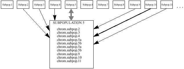Figure 5. Baluja's architecture of subpopulations, arrangement #3. Subpopulation 5 is shown enlarged.

• This last algorithm is an implementation of a diffusion model GA. It was proposed by White and Pettey at [WP97]. The diffusion model GA typically maps each individual in the population to a different process. Each process is then executed on its own processor. In order to perform selection and crossover, each process must communicate with other processes to gather information about other individuals. This communication causes overhead that slows down the execution of the GA. Thus, selection and crossover are usually performed with the knowledge of only a subset of the population, often called the neighborhood.