The Time Series Identification Problem


Description:
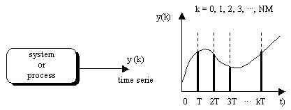
System Identification (SI) [1] tries to find a parametric model of dynamical systems from its input and output (I/O) measured values. We work with Time Series (TS), which can be considered as single output sampled systems with period T:

The parametric polinomial ARMAX modelation [2] of these time series is described in the following equations. The serie is the y signal. With the obtained model of the time serie we can determine the estimated signal (ye), and then to compute the generated error.


For determining the parameter vector (the model) we consider recursive estimation, that updates q in each time k, modelling so the system. To more sampled data processed, better precision for the model because it has more information about the system behaviour history. We consider SI performed by the well known Recursive Least Squares (RLS) with forgetting factor algorithm [3]. From the initial conditions, we start building the data vector, then:

This algorithm is specified with ff (the forgetting factor, many time denoted with the lambda character), initial values and the observed signal {y(k)}. There is not any fixed value for ff, even it is used a value between 0.97 and 0.995 [4]. The cost function F is defined as the value to minimize:
![]()
The recursive identification is very useful for predicting the system behaviour when there is a high degree of complexity and variability in the response. So, it is necessary to elaborate a mathematical model for covering the system behaviour. As identification advances in the time, the predictions improve using more precise models. For example, we can compute in sample time the system model and then, with this model to simulate the system future behaviour, forwarding real situations.
The optimization problem:
We are interested in the system behaviour prediction in running time, that is, while the system is working and its signal is being observed. At the same time, our first effort is to obtain high model precision (minimal F). The precision is due to several causes, mainly to the forgetting factor ff. There is not any determined value for ff, but it is usually used within 0.995 and 0.98 [2][4]. Frequently this value is critical for model precision. Other sources also can have certain degree of influence (dimensions, initial values, the system...). Also, it may appear the precision problem when the system response changes quickly. Then the sample frequency must be high for avoiding the key data lost in the system behaviour description, and this implies a computational cost. We find the trade-off between a high sample frequency and a high precision in the algorithm computation. By that, it is interesting to research about algorithms for finding the best ff values for each system. In relation with the model dimensions, we can say that for a dimension of reasonable computational cost, ff is the most important optimization parameter.
Related Papers:
[1] Söderström et al., T:
“System Identification”. Prentice-Hall, London (1989)
[2] Ljung, L: System Identification – Theory
for the User. Prentice-Hall, London (1999)
[3] J.E. Parkum: “Recursive Identification of
Time-Varying Systems”, Ph.D. thesis, IMM, Technical University of
Denmark (1992)
[4] Ljung, L: System Identification Toolbox. The Math
Works Inc. (1991)
![]()
Last Updated:
5/5/03
For any question or
suggestion, click here to contact
with us.